InferTheta is a decision infrastructure platform that uses probabilistic graphs and Bayesian inference to govern AI agents and autonomous hardware.

How to use the software in everyday language — from Bayesian networks and inference to learning, decisions, and the editor.

This guide explains InferTheta in everyday language. You do not need a background in Bayesian networks, statistics, or data science to follow it. Technical words are introduced only when useful, and always with a simple meaning.

Think of InferTheta as a visual workspace where you draw how things influence each other, tell the software what you currently know, and see how likely other things become. You can also learn those relationships from spreadsheets or data files, compare decisions, and export your model for sharing or use in other systems.

1. What Bayesian networks / Probabilistic graphs are (simply put)

InferTheta is built on Bayesian networks (also called Probabilistic graphs or causal networks). The platform allows engineers, AI researchers and data scientists to design, train and deploy their causal AI models easily without doing a single line of code using both their expert knowledge and data. The whole basic idea behind such models is the capacity to answer questions such as:

• Given what I know about something, what is the probability that X happens?
• Given I know (or assume) X will happen, what are the most likely causes?

This section explains the idea without assuming any specialist background.

Nodes, edges, and uncertainty

A Bayesian network is a diagram of uncertain quantities. Each box (node) is something that can take different values — for a loan application that might be Employment stability (Stable / Unstable), Payment history (Clean / Missed payments), and Default risk (Low / Medium / High).

An arrow from A to B means “A helps explain B” — often read as a direct influence or cause. For example, Employment stability → Default risk says that how stable someone’s job is matters for how likely they are to default. Knowing employment can change what you believe about default, even before you see anything else.

Importantly, the graph must stay free of loops: you cannot have a path of arrows that comes back to the same node (A → B → C → A). That acyclic rule is what lets the mathematics stay coherent. InferTheta blocks links that would create such a loop. If you want a loop, you need to create a Markov Chain, which is also possible with InferTheta.

Why the diagram saves so much work

In principle, any set of Yes/No (or multi-state) variables has a giant joint table: every combination of all variables at once. With only a handful of binary variables that table is already large; with dozens it becomes impossible to fill by hand.

A Bayesian network replaces that giant table with many small tables. Each node only stores how it depends on its direct parents (its incoming arrows). Nodes with no parents store a simple prior (“before we know anything, how likely is Stable employment?”). Missing arrows encode independence: if two nodes are not connected (and not linked through a shared path you care about), the model treats them as not directly informing each other.

Lending example. Suppose Default risk depends on Employment stability and Payment history, and Payment history depends on Employment stability, but we decide Payment history does not need a direct arrow from some unrelated field such as Preferred branch colour. By omitting useless arrows, we keep the model small enough to understand, review, and compute.

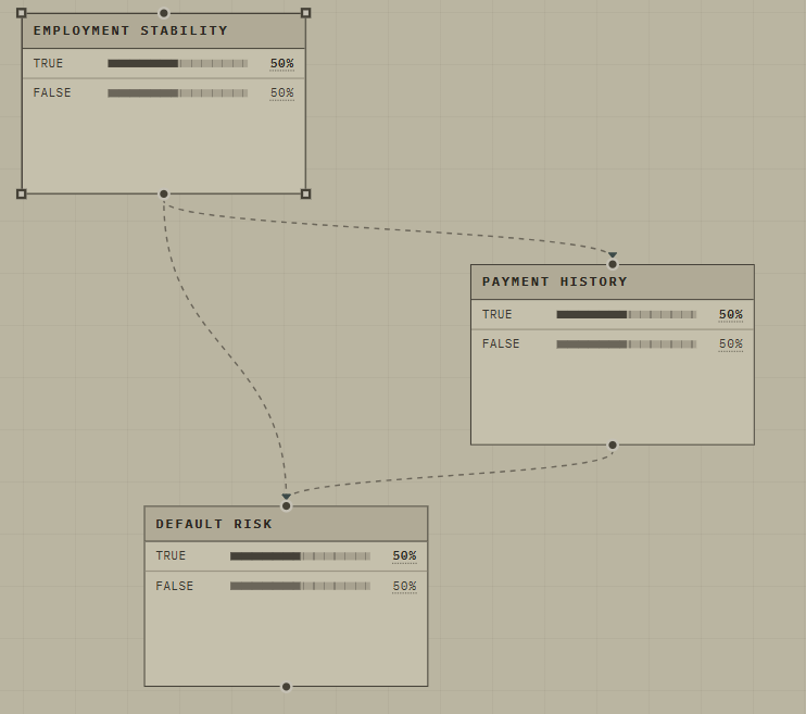
This is very important for models that need to make inferences at the ms because they are embedded in products or hardware.

Two ways to read the same diagram

Formally, the network is a factorization of a joint probability distribution: the full story of all variables together is the product of each node’s local table given its parents. Different arrow layouts correspond to different factorizations of the same kind of story.

In practice, most people also read arrows causally: “employment influences payments, and both influence default.” That informal reading is extremely useful for building models with experts. When in doubt, draw the influences you believe exist, then check that the numbers and independence assumptions still make sense.

Reading the CPTs and making inference based on observations

Instead of bombarding you with complex probability theory, we will go through an example.

Here is a very simple Bayesian network (source: Koller & Friedman, Probabilistic Graphical Models, 2009) that gives the probability of getting a strong letter of recommendation depending on certain variables.

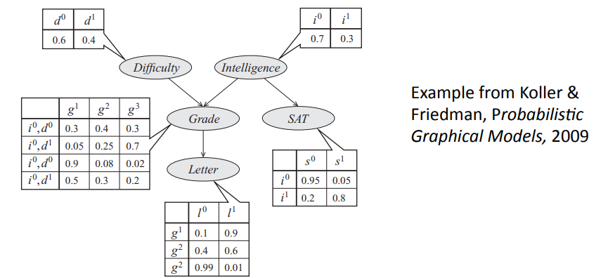
You notice that each row sum to 1 because it gives you cover all the alternatives. For instance, given I am not very intelligent (i0), but the exam is not difficult (d0), the probability of getting grade 1 is 0.3, grade 2 is 0.4 and grade 3 0.3. The tables are the CPTs of each node given their parents.

Now, how do we computation based on what we (don’t) know. Let’s say, if we know the student is intelligent (i1), what is the probability they get a strong letter (l1)?

You will notice that we don’t know anything about the grade itself. But we do know the CPT of the grades given difficulty and intelligence. We also know the probability of getting a strong letter depending on the grade, it’s the l1 column (0.9 ; 0.6 ; 0.01). With all of that, we can do something called “Averaging”.

Step-by-step: averaging to get the prior P(L = Strong)

Before we put evidence on Intelligence, it helps to compute the baseline: with no observations, what is P(Letter = Strong)? Letter depends only on Grade, so we use the law of total probability (averaging):

P(L = Strong) = 0.9 × P(G = A) + 0.6 × P(G = B) + 0.01 × P(G = C).

We do not observe Grade either, so we must first average the Grade CPT over Intelligence and Difficulty (independent roots: P(I = Low)=0.7, P(I = High)=0.3, P(D = Easy)=0.6, P(D = Hard)=0.4).

Averaging step 1 — prior grade probabilities

P(G = A) = 0.30×0.7×0.6 + 0.05×0.7×0.4 + 0.90×0.3×0.6 + 0.50×0.3×0.4 = 0.126 + 0.014 + 0.162 + 0.060 = 0.362.

P(G = B) = 0.40×0.7×0.6 + 0.25×0.7×0.4 + 0.08×0.3×0.6 + 0.30×0.3×0.4 = 0.168 + 0.070 + 0.0144 + 0.036 = 0.2884.

P(G = C) = 0.30×0.7×0.6 + 0.70×0.7×0.4 + 0.02×0.3×0.6 + 0.20×0.3×0.4 = 0.126 + 0.196 + 0.0036 + 0.024 = 0.3496.

Check: 0.362 + 0.2884 + 0.3496 = 1.

Averaging step 2 — mix with the Letter CPT

P(L = Strong) = 0.9×0.362 + 0.6×0.2884 + 0.01×0.3496 = 0.3258 + 0.17304 + 0.003496 = 0.502336 ≈ 0.50.

So without any evidence, a strong letter is about a coin flip. That 50% is not a single CPT cell — it is two layers of averaging: first over (I, D) to get P(G), then over G to get P(L).

Forward inference example (cause → effect)

Question: if we know the student is intelligent (I = High), what is P(L = Strong)? Information flows along the arrows: Intelligence → Grade → Letter.

First update Grade given I = High (still averaging over Difficulty):

• P(G = A | I = High) = 0.9×0.6 + 0.5×0.4 = 0.74
• P(G = B | I = High) = 0.08×0.6 + 0.3×0.4 = 0.168
• P(G = C | I = High) = 0.02×0.6 + 0.2×0.4 = 0.092

Then push that through the Letter CPT:

P(L = Strong | I = High) = 0.9×0.74 + 0.6×0.168 + 0.01×0.092 ≈ 0.77.

Compared with the prior ≈ 0.50, knowing the student is intelligent raises the chance of a strong letter to about 77%. That is forward inference: evidence on a cause updates beliefs about effects.

Even shorter forward check from the SAT CPT alone: P(S = High | I = High) = 0.8 (no averaging needed — Intelligence is the only parent).

Backward inference example (effect → cause)

Question: we only observe SAT = High. What is P(I = High)? The arrow is Intelligence → SAT, but evidence on the child updates the parent (diagnosis).

From the SAT CPT: P(S = High | I = Low) = 0.05 and P(S = High | I = High) = 0.8. First the marginal of the evidence:

P(S = High) = 0.05×0.7 + 0.8×0.3 = 0.035 + 0.24 = 0.275.

Then Bayes’ rule:

P(I = High | S = High) = [P(S = High | I = High) × P(I = High)] / P(S = High) = (0.8 × 0.3) / 0.275 = 0.24 / 0.275 ≈ 0.87.

Prior intelligent = 30%; after a high SAT ≈ 87%. That is backward inference: evidence on an effect revises beliefs about its causes.

Summary of the two directions

• Forward (I = High → L = Strong): prior ≈ 50% → about 77%.
• Backward (S = High → I = High): prior 30% → about 87%.

InferTheta does these updates automatically when you set evidence on the canvas; the point of the hand calculation is to see that the on-screen percentages come from averaging CPT rows (forward) or from Bayes’ rule (backward), not from reading one CPT cell in isolation.

That being said, that example should make one thing clear: probabilistic inference gets hard fast. Even a five-node textbook network already needs careful averaging and Bayes’ rule. With hundreds of nodes, many states, and dense parent–child links, coding this would be tedious, error-prone, and effectively impossible for anyone who is not deeply trained in probability.

That is why InferTheta matters. It does the calculations for you, and—just as important—it shows why numbers move (evidence, CPTs, contributions). So, people with limited formal background can still build causal / probabilistic AI models and remain able to explain and audit what the model is doing.

What you do with a finished network

Once structure and tables are in place, you reason by setting evidence — marking what you currently know (for example Payment history = Missed payments). InferTheta then updates beliefs on the other nodes (for example Default risk rises). That update is probabilistic inference: it applies the rules of probability consistently across the whole diagram, not just the nodes you clicked.

Below, on the right, you have the probabilities without any knowledge of a bank customer. On the right, you know they have missed a payment before. You will notice that this gives you info not only about the default risk, but also about their employment stability.

That is why InferTheta feels like a living calculator: change what you know, and related probabilities move in a principled way.

2. The big picture in one minute

In InferTheta, a model is a diagram made of nodes (variables) and edges (influences).

• A node is something that can take different values — for example “Customer pays late?” with Yes / No, or “Fraud risk” with Low / Medium / High.
• An edge from A to B means “A helps explain B” or “B is caused by A” Knowing something about A can change what you believe about B. This is also why Probabilistic graph modelling is also referred to as “Causal AI”. If you learn relationships from variables, you can understand and explain what causes what.
• When you mark something as known (called “setting evidence”), InferTheta updates the probabilities on the other nodes to match that information.
• If you add decisions and utilities (payoffs), You can suggest which action looks best under uncertainty.

3. Getting started

Sign in

Where to find it: The login screen when you open the app; once signed in, your account controls sit on the right of the toolbar.

What it does: InferTheta asks you to sign in so your workspace is protected. Depending on your organization, you may also manage billing from here.

Why use it: Keeps access controlled and lets you return to your work securely.

Network title

Where to find it: Toolbar, second row — the text field that often says “Untitled network”.

What it does: Gives your model a human-readable name. That name is reused when you save or export files.

Why use it: Makes it easy to find the right model later among many files.

New network

Where to find it: Toolbar → New network.

What it does: Clears the canvas so you start from a blank model. If you have unsaved changes, InferTheta asks before discarding them. Make sure to either save on the browser or export a json file version of the network if you want to get back to it later.

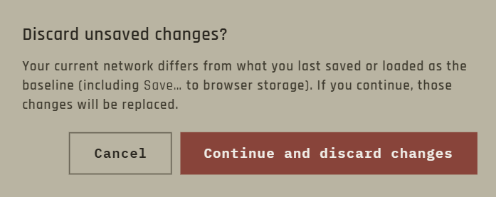
Why use it: Useful when you want a clean slate without leftover boxes from a previous example.

Save and Open (browser library)

Where to find it: Toolbar → Save… and Open saved.

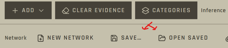
What it does: Stores models in this browser on this computer, and lets you reopen or delete them later. You can also save a copy under a new name.

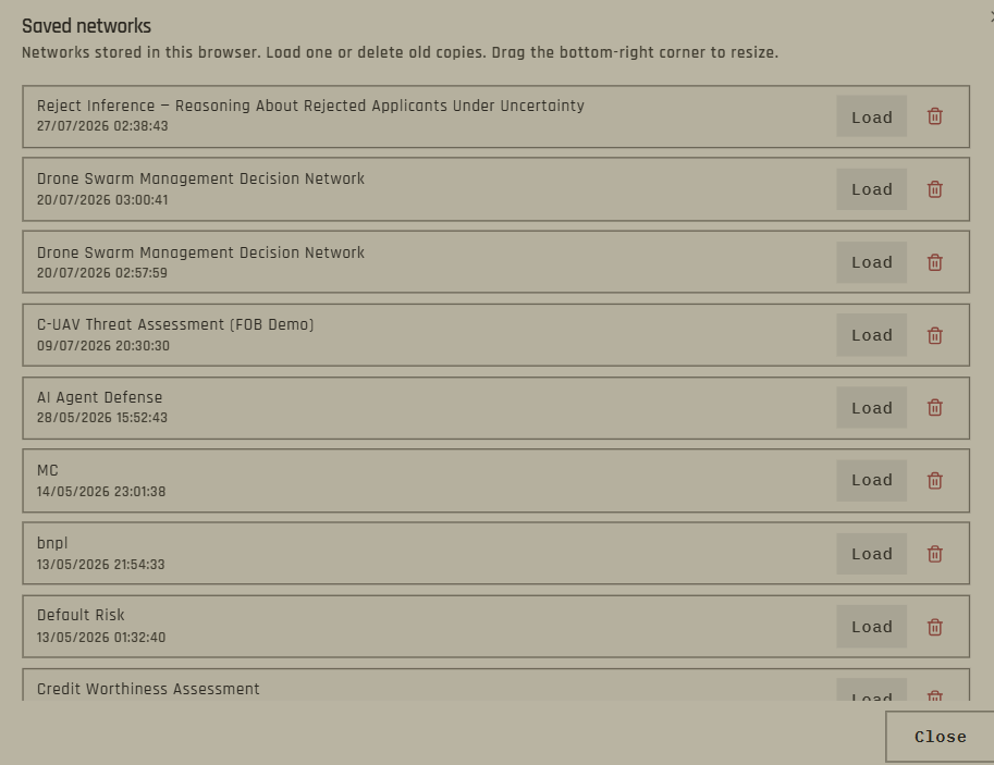
Careful with the webapp version! Networks are linked to the browser on the machine you use, not your account. If you work across different machines, make sure to export the json file to get back to it easily.

Why use it: Quick local backup while you work — no need to download a file every time. For sharing across machines, use Export (see later).

Snapshot and Restore

Where to find it: Toolbar → Snapshot / Restore.

What it does: Takes an in-memory checkpoint of the current diagram in this browser tab, and can restore it. Reloading the page clears the snapshot.

Careful! This is not a substitute for saving the network. Think of it more as a way to momentarily capture that specific configuration of the network and easily come back to it after some edits if needed (Think of “save states” when emulating video games on PC).

Why use it: Safe way to try a risky edit: snapshot first, experiment, restore if you dislike the result.

4. Build a model

Everything starts with the Add menu on the toolbar. You place nodes on the canvas, connect them with arrows, and fill in what each box means.

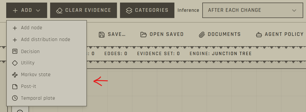
4.1 Types of nodes you can add

Chance node (ordinary variable)

Where to find it: Toolbar → Add → Add node.

What it does: A standard uncertain variable with named states (for example Low / Medium / High) and a table of probabilities (its CPT — “conditional probability table”).

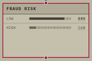
You edit the name, states, and table in the right-hand configuration panel that appears whenever you select a node.

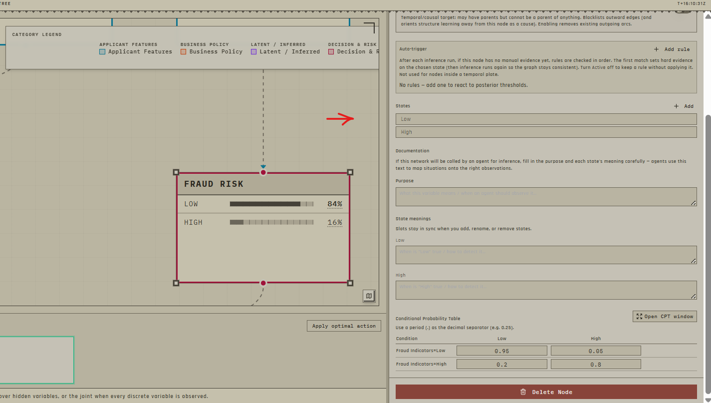
Why use it: This is the workhorse for most business and risk questions: anything that is uncertain and can be described with a few clear categories. Although quite simple in appearance, this type of causal modelling can be incredibly powerful when capturing complex conditional dependencies, non-linear relationships, and real-world uncertainty. In practice, most real-world probabilistic graphs are built exclusively with discrete multi-state nodes. The specialized nodes below address niche, complex scenarios and are best suited for advanced modeling needs.

Distribution node

Where to find it: Toolbar → Add → Add distribution node, then choose a distribution type.

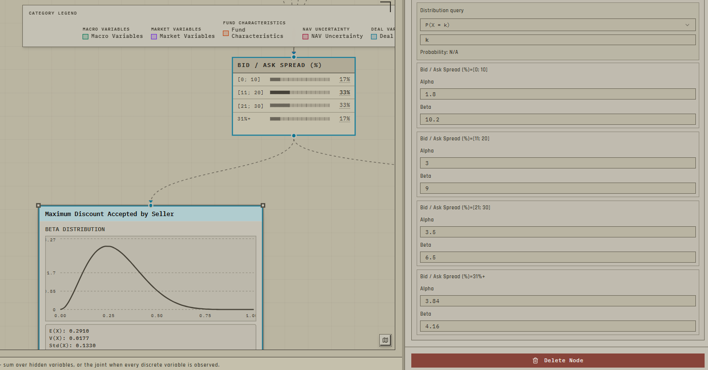
What it does: A variable described by a continuous or parametric law (for example Normal, Beta, Gamma) instead of a short list of labels. You can plot it, query ranges, and optionally link it to other variables (discrete or continuous).

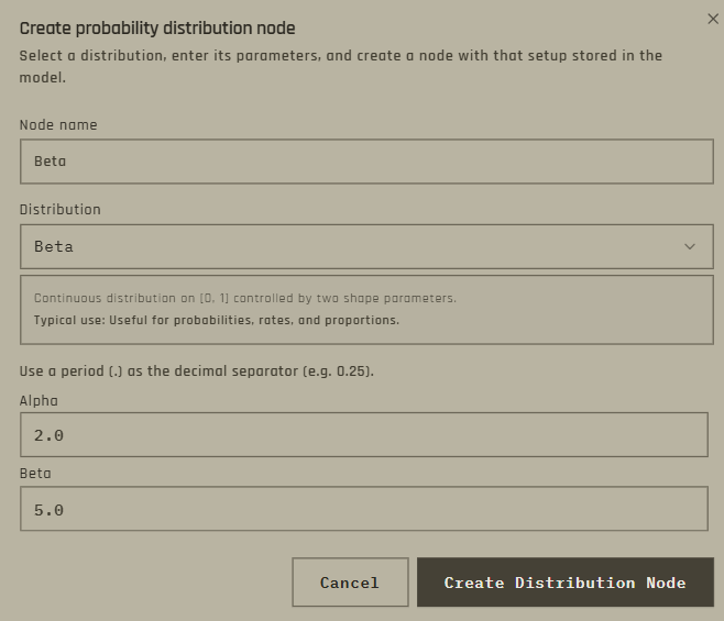
Why use it: Use this when the quantity is naturally numeric (amounts, rates, sizes), a few labels would be too coarse, and you know a certain type of probability distribution would fit the situation better. For instance, if you want to do what-if simulations about a rate, you will need a number between 0 and 1, you can use a beta distribution and condition its parameters depending on certain variables.

Decision

Where to find it: Toolbar → Add → Decision.

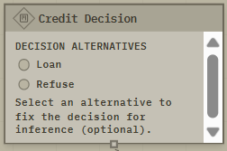
What it does: A box that represents a choice you control — for example Investigate / Clear / Freeze — not something random. You list the alternatives in the sidebar.

Two main use cases for using Decision nodes.

Why use it: Needed whenever the question is “What should we do?” rather than only “What is likely?” This type of node can only be a parent, not a child. Two main use cases for using Decision nodes.

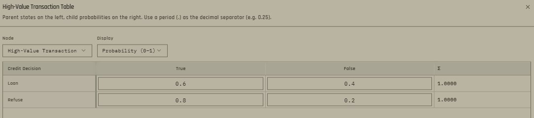
First one is to make simulations based on decisions: “if I decide to do X, what happens?” or “If X happened, what are the most likely causes?”

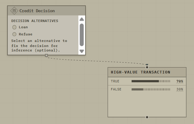
The CPTs of the discrete nodes will be conditioned by the decisions from the decision node

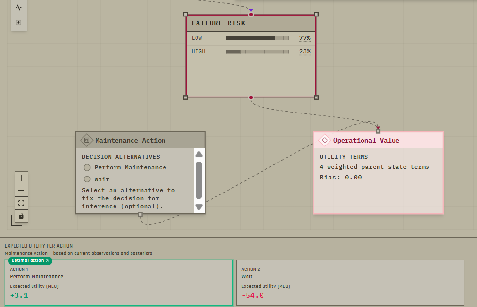
Second one is to link decision nodes and make them parents of a utility node (see below) to propose a recommendation based on observations made. In this case, selecting a decision will not influence anything on the network as it is the output.

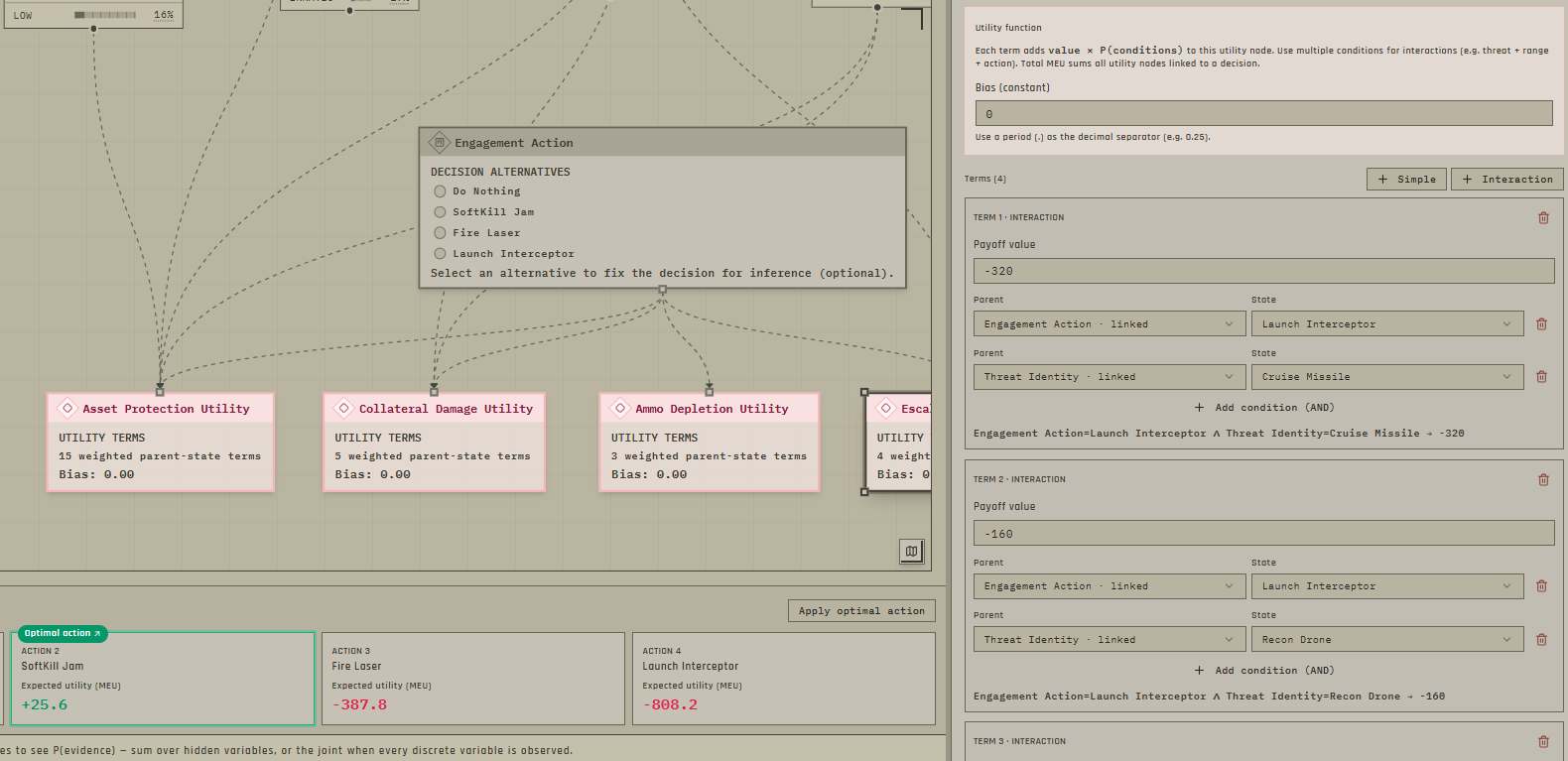
Utility

Where to find it: Toolbar → Add → Utility.

What it does: A scoreboard for how good or bad outcomes are (costs, rewards, preferences). You define payoff terms in the sidebar, often depending on decisions and chance variables. They need to have a decision node as parent.

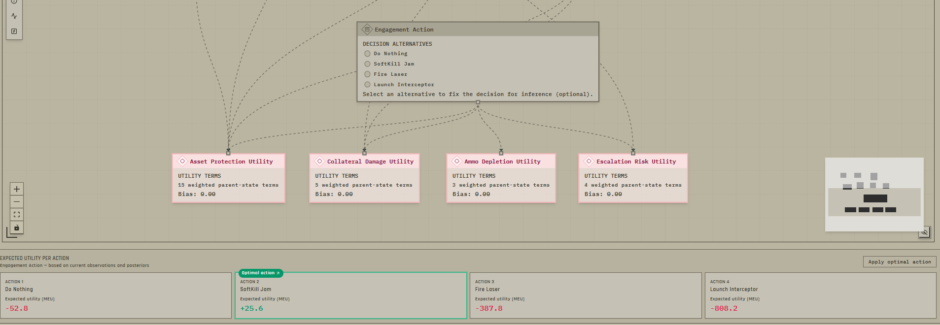
Why use it: This let you recommend certain actions and decisions to make depending on what you know about certain variables. You can directly input the payoff of the utility function to favor / prevent certain decisions depending on the status of the parent variables.

Markov state

Where to find it: Toolbar → Add → Markov state.

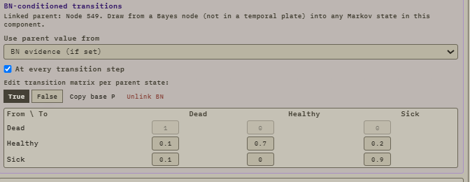
What it does: A state in a step-by-step process (healthy → sick → recovered, or application stages). You can mark a state as absorbing (terminal). Transitions are edited on the arcs and in the Markov panel.

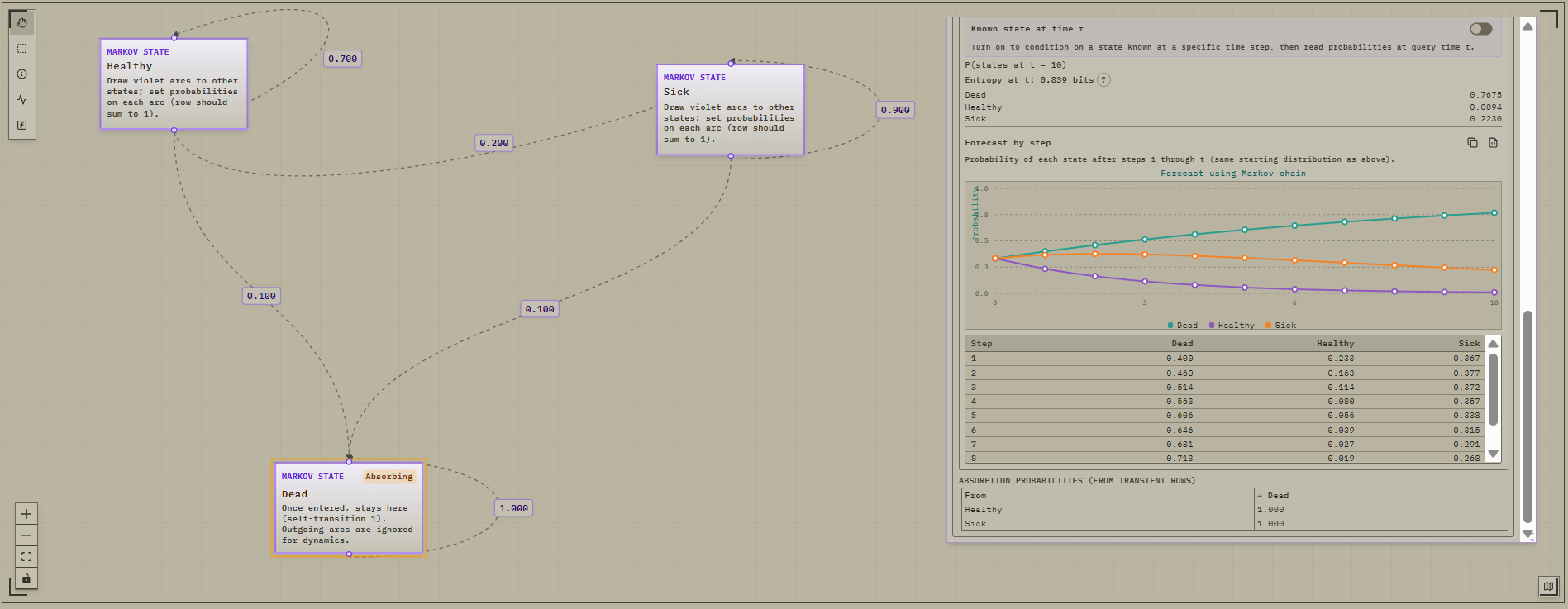
Just like graphs, you can learn Markov chains directly from data if you structure your data the following way:

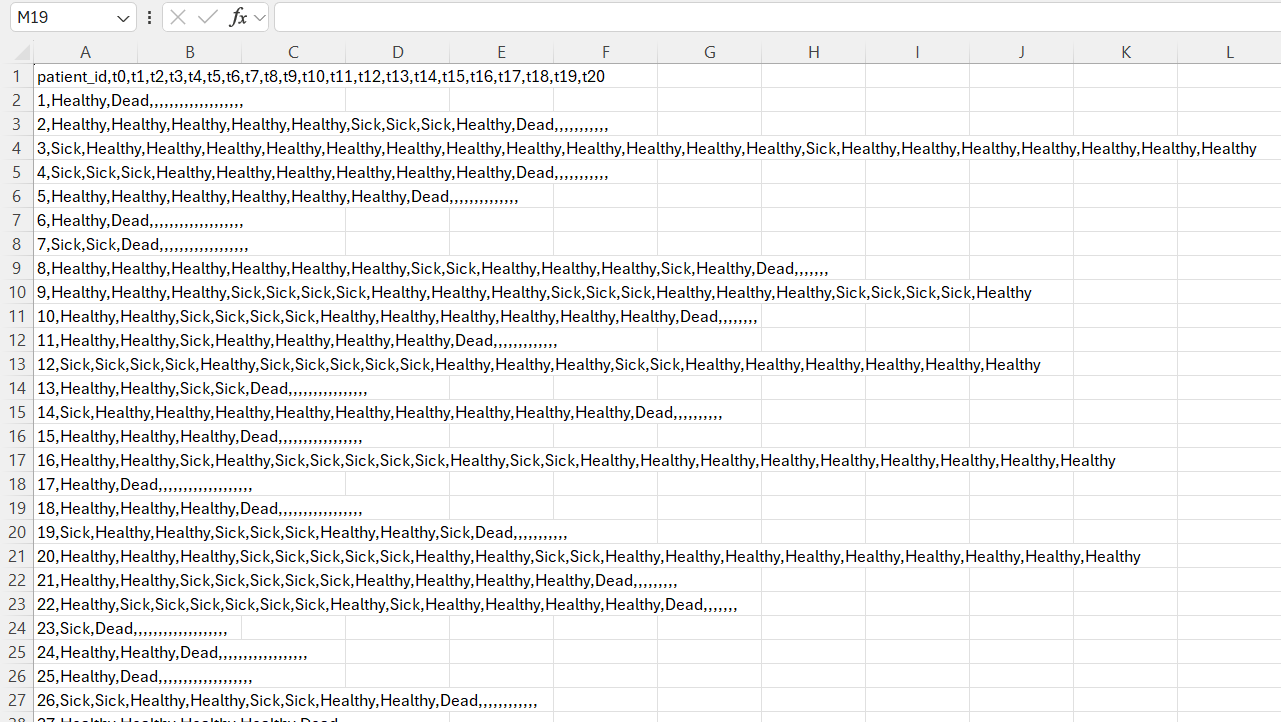
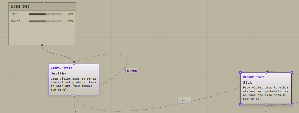
Why use it: Useful for workflows and processes that unfold over stages or time steps. You can also condition your Markov chain to a node, with its values changing depending on the state the node takes.

Post-it

Where to find it: Toolbar → Add → Post-it.

What it does: A sticky note on the canvas for comments and reminders. It does not participate in calculations.

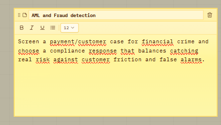
Why use it: Capture assumptions, open questions, or stakeholder notes next to the model. This is mostly useful to give context to people discovering the model about its variables, its structure, the parameters and how it has been designed.

Temporal plate (advanced)

Where to find it: Toolbar → Add → Temporal plate.

What it does: A framed region that says “these variables repeat over several time steps.” Nodes whose centers sit inside the plate become templates across time (a dynamic network). This allows simulations such as “Given what I know at t = 2, what is the probability of X at t = 5 for instance”. This type of modelling is called dynamic Bayesian network.

Membership rule: a discrete chance node is temporal if its center sits inside the plate. Resize/move the frame so the right nodes are inside.

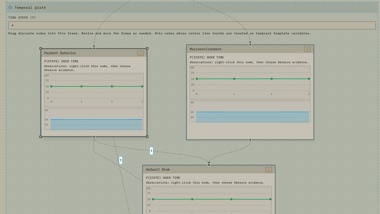
Basically, you draw the network once. InferTheta treats it as a compressed template for a longer story: the same variables at time 0, 1, 2, … up to T − 1. Under the hood it “unrolls” that template into many linked copies — without you drawing Customer Risk_t0, Customer Risk_t1, Customer Risk_t2 etc. by hand.

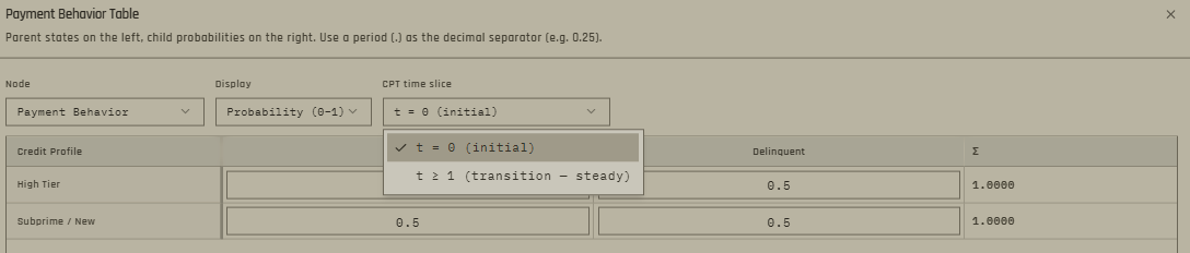
You will have to fill in a CPT for each time t.

Instantaneous vs temporal (lag)

Click an arrow between plate variables (or a self-loop) and set Dependency:

Setting

Meaning

Instantaneous (lag 0)

Same time step: A and B influence each other within one period.

Temporal (lag ≥ 1)

Across time: parent at time t influences child at t + lag.

Lag = how many steps the influence is delayed. Lag 1 = “yesterday → today.” Lag 2 = “two periods ago → today.”

Self-loops (arrow from a node to itself) are always temporal (default lag 1). Instantaneous self-loops aren’t allowed — that would be a cycle inside one time slice.

That’s why self-loops matter for self-reinforcing stories: “Fraud Risk_t depends on Fraud Risk_{t−1}.”

Why use it: Model sequences — this week / next week / later — without redrawing the whole diagram for every period. Use a temporal plate when today affects tomorrow — especially:

• Self-reinforcing / persistent phenomena — risk stays high because it was already high; trust builds only gradually; an account “warms up” into fraud after several odd steps.
• Delayed effects — a signal today changes a state next period (lag ≥ 1).
• Sequences of observations — you learn more over days/weeks and want beliefs to update along that timeline.

Skip it for one-shot cases (single transaction, single claim) with no meaningful “next period.”

Careful for webapp users! Temporal plates can easily cause an explosion in “hidden nodes” and doing inference in the browser will become laggy. It’s better to stick to a few nodes within a temporal plate, and avoid making too big.

4.2 Connecting nodes (edges)

Draw an influence edge

Where to find it: On the canvas, drag from a connection point on one box to another. You need to drag from the bottom of a node to the top of another to create a parent / child relationship. You can identify which node is the child by looking for an arrow near the top of the node.

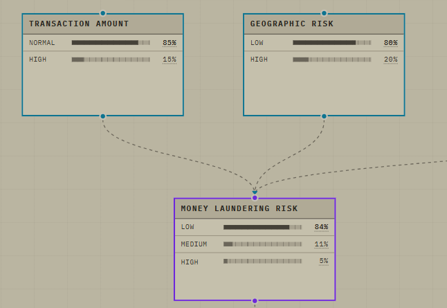
What it does: Creates a directed link: the source is a “parent” that helps explain the target (“child”).

Why use it: Without edges, nodes are independent. Edges are how you encode domain knowledge about what affects what.

For instance, in the example above, Transaction Amount and Geographic Risk are considered independent from each other, but are parents of the node Money Laundering Risk. This means that the probabilities shown in Transaction Amoun and Geographic Risk are directly from their CPTs since they have no parents, but the ones shown in Money Laundering Risk will directly be influenced by the observations (not) made in the parent nodes (so it’s always a result of probabilistic inference).

Reverse or configure an edge

Where to find it: Click an edge, then use the edge controls that appear.

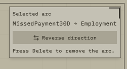
What it does: You can reverse direction. For temporal models, you can choose whether the link is instantaneous or crosses time steps (with a lag).

Why use it: Fixes mistakes quickly and supports time-lagged stories (cause today, effect tomorrow). This is mostly useful when you learn learn graphs directly from data, and the AI identify a causal relationship between variables that makes sense only the other way around. For instance, the AI correctly identifies a causal relationship between the stability of employment of someone, and their payment history of the last 30 days, but the edge is from missed payments to employment. Obviously, it should be the other way around so this option allows you to quickly correct the AI. This happens because data mostly shows that two things move together, not which one causes which. From correlations alone, “missed payments ↔ unstable employment” looks almost the same either way, so the learning algorithm sometimes draws the arrow backwards.

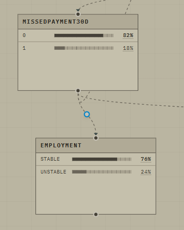
Good practice! When you are done learning relationships and switching edgdes, always select “Re-learn parameters” at the bottom right of the screen in design from data mode (you know you are in this mode because you have a yellow border on the canvas). This will allow the AI to adjust the parameters to the causal relationship you impose.

See strength

Where to find it: Canvas controls (top-left area).

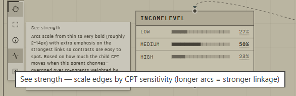
What it does: Thickens arrows based on how strongly the child’s probability table depends on that parent.

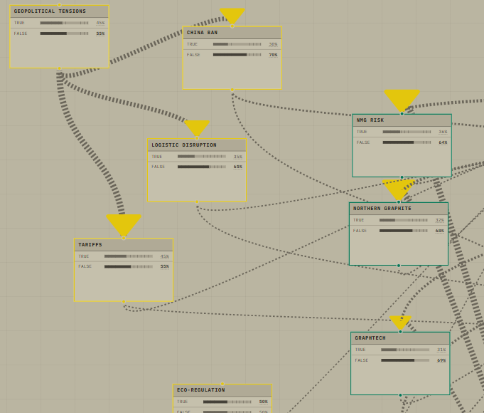
Why use it: Helps you spot the most important relationships visually in a busy diagram.

4.3 Editing what a node means

Node configuration sidebar

Where to find it: Click a node; the panel opens on the right.

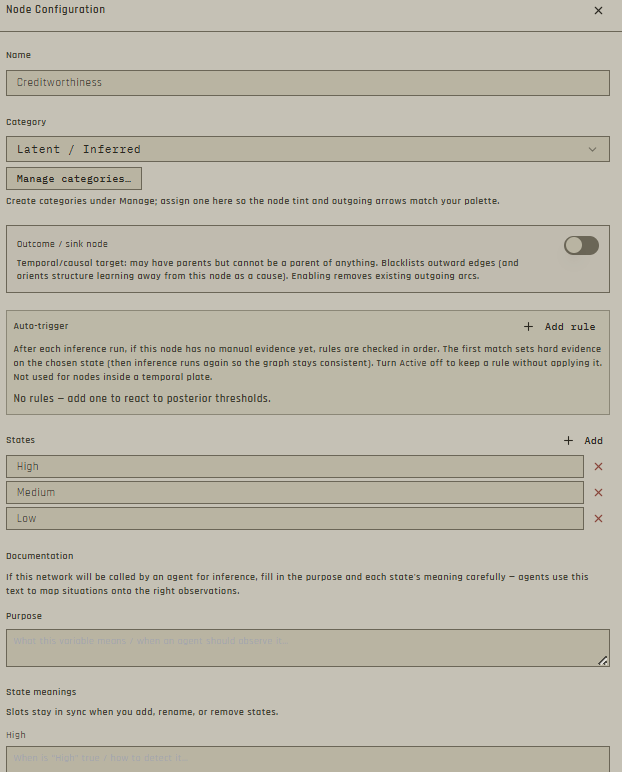
What it does: Rename the variable, change its category color, edit states or decision alternatives, edit probability tables, write documentation, configure distribution settings or utility terms, and delete the node.

Why use it: This is the main place to fully define each piece of your model.

CPT editing (probability tables)

Where to find it: Sidebar table, or open the larger CPT window from the sidebar.

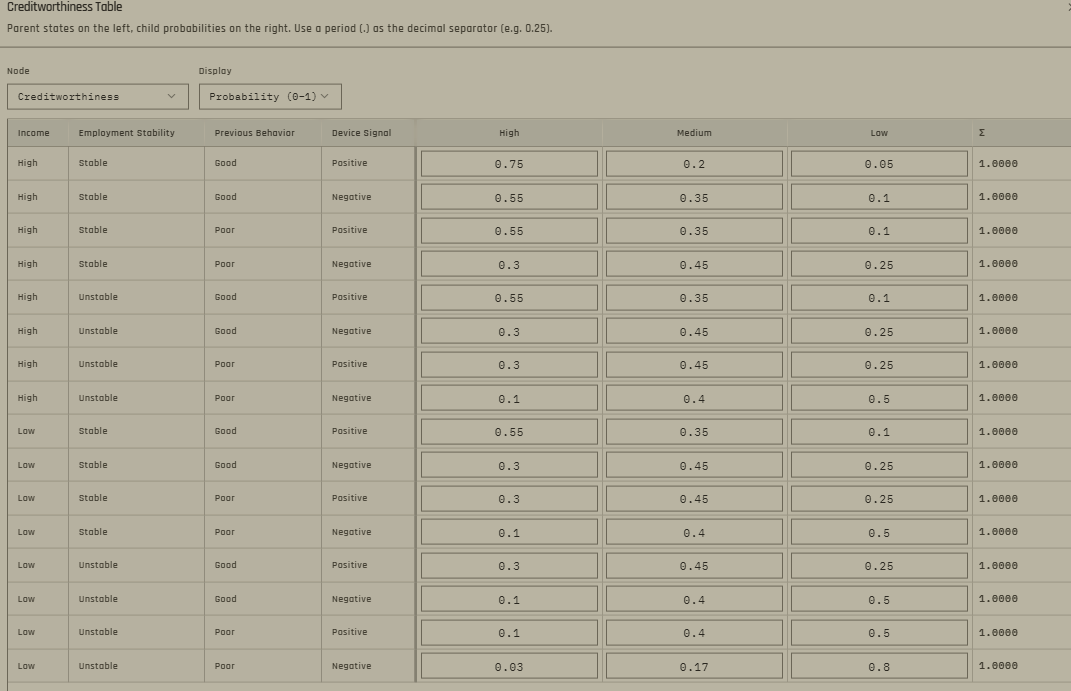
What it does: For each combination of parent values, you set how likely each child state is. Rows should add up to 100%. You can display values as percentages or probabilities.

Why use it: This is where expert knowledge lives: “When income is High and history is Clean, default risk is mostly Low.” This is your main way of inserting Intuition / Expert knowledge into your model when you are not learning directly from data. This allows you to not be blocked and make assumptions. You can then test your assumptions with experimentations and update those parameters when you do start collecting data.

Categories and legend

Where to find it: Toolbar → Categories; also category pickers on nodes; floating legend on the canvas.

What it does: Create color groups (for example Fraud / Customer / Controls) and assign nodes to them. Edges can tint by the source category.

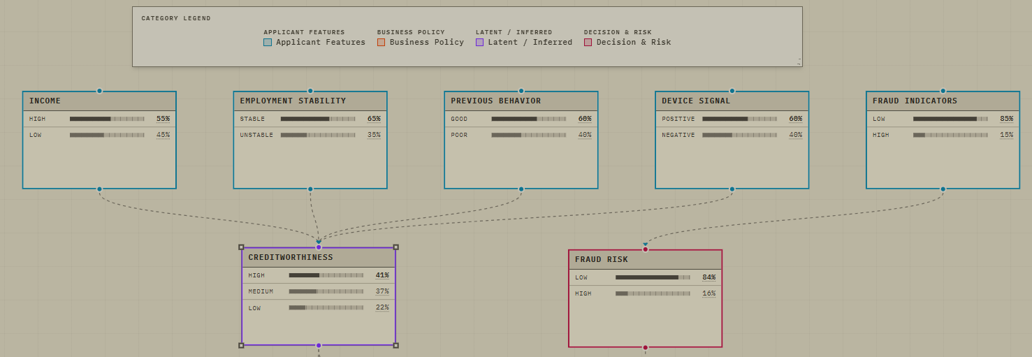
Every time you add a node to your graph, you will have the option to assign it a category on the right-side editor.

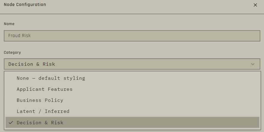
Why use it: Large models stay readable when related boxes share a visual identity.

Outcome sink

Where to find it: Toggle in the sidebar on a chance node.

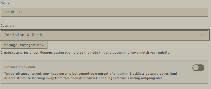
What it does: Marks a variable as an end target: it can have parents, but it cannot point to other variables.

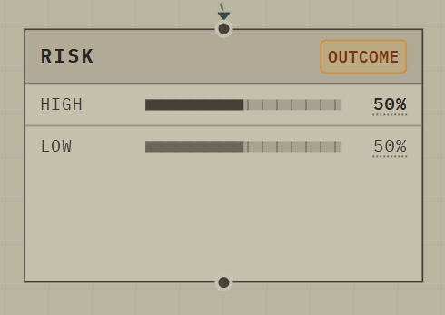
Why use it: Useful for outcomes you want to predict (default, fraud, repayment) without accidentally feeding them back into predictors. This can be important when learning relationships from data. By designating this node as end-target, you make sure the AI considers that when proposing graphs and will not make this node a parent to any other variables. If it finds relationships, it will understand it is necessarily a child node.

Documentation on nodes

Where to find it: Sidebar → Documentation.

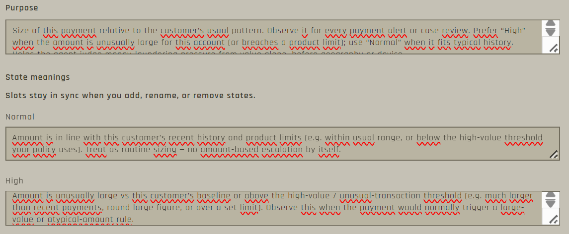
What it does: Write what the variable means and when each state should be used. This travels with the model and can help people or automated assistants interpret it correctly.

Why use it: Avoids ambiguity like “High risk — according to whom?” when someone else opens your network later. This is also really important if the model is destined to be used by LLM-powered agents, as that will help them making correct observations within the graph. Even if the model is going to be used only by people, it can help for compliance purposes.

Derive a random variable (convolution)

Where to find it: Canvas toolbar function control (after selecting several Bayesian nodes).

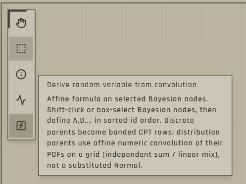
What it does: Creates a new variable from a simple formula on selected parents (for example a weighted sum), as either bins or a continuous combination.

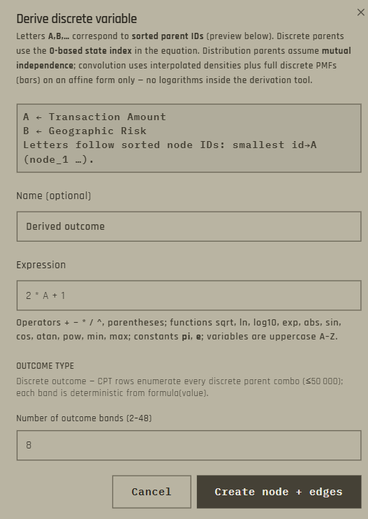
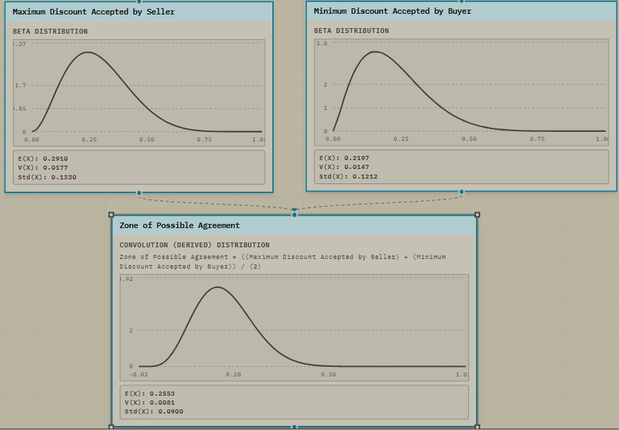
Example above is an example of convolution created from two previous provability distributions, and all three automatically updates depending on the observations made in the network. The formula is always displayed when a distribution is the result of a convolution (in this example: Zone of Possible Agreement = (Maximum Discount Accepted by Seller + Minimum discount Accepted by Buyer) / 2)

Why use it: Combine existing uncertainties into one quantity without building huge tables by hand, and keep that derived law in sync with the rest of the model.

Copy and paste nodes

Where to find it: Right-click a node → Copy; paste on the canvas.

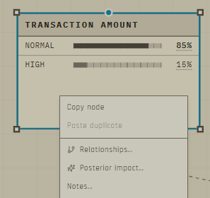
What it does: Duplicates selected nodes so you can reuse structure.

Why use it: Speeds up building repeated patterns.

Delete a node

Where to find it: Select one or more nodes on the canvas, then press Delete (or Backspace) on the keyboard. You can also delete the selected node from the right-hand configuration sidebar (Delete Node).

What it does: Removes the node and its attached edges from the model.

Why use it: Fast cleanup while editing. Tip: click the canvas background first if a text field still has focus, so the keypress is not typed into a label instead of deleting the node.

Right-click menu on a node

Where to find it: Right-click (or two-finger click) a node on the canvas. The exact items depend on the node type.

What it does: Opens a short menu of actions without opening the full sidebar.

Chance nodes (discrete Bayesian nodes) typically offer:

• Observe evidence… — for nodes inside a temporal plate: set observations at different time steps.
• Clear evidence — remove a hard observation from this node (shown when evidence is set).
• Copy node / Paste duplicate — duplicate nodes (and paste a previously copied selection).
• Relationships… — inspect which nodes are parents or children of this one.
• Posterior impact… — see how candidate observations on related nodes would move beliefs.
• Notes… — open documentation / notes for the node.

Decision and utility nodes mainly offer Copy / Paste duplicate and Inspect in sidebar (opens the configuration panel). Markov states offer Copy / Paste. Post-its offer Copy / Paste.

Why use it: Quick access to evidence, documentation, and analysis tools without hunting through the toolbar.

Canvas navigation

Where to find it: Pan / box-select controls, zoom, optional minimap.

What it does: Move around large diagrams and select many nodes at once.

Why use it: Essential once models grow beyond a handful of boxes. Tips! Sometimes you might lose your nodes on the canvas because you are too far away from them. Just use the minimap on the bottom-right corner to locate them. You can always hide it again after.

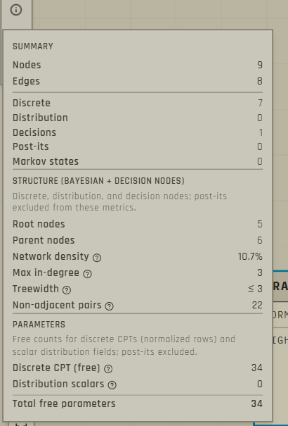
Network summary

Where to find it: Info popover on the canvas controls.

What it does: Shows counts of node types and simple complexity indicators.

Why use it: Helps you judge whether the model is getting large before updates feel slow.

5. Ask questions: evidence, scenarios, and inference

Building the diagram is only half the story. The power of InferTheta is asking “what if we know this?” and watching beliefs update. This allows you to see what will happen when you use this model for an API call, an agent use it for making observations before taking decisions, or your autonomous hardware reasons under uncertainty.

Set evidence on a chance node

Where to find it: Click a state bar on the node (or use the sidebar).

What it does: Marks that state as observed (“we know this is Yes”). Other nodes update their probabilities. Click again (or clear) to remove the observation. You can observe as many evidence as you want and clear them all at once with the “Clear evidence” button.

Why use it: This is how you condition the model on real information: a transaction flag, an interview answer, a sensor reading, and so on. Inference will always be done forward and backward, meaning if you make an observation on a node that has children, the probabilities of the different states of those children will update. And if they have parents, this will also update the probabilities of the different states of those parents.

In the example below, on the left you can see the probabilities regarding the money laundering risk given we know nothing about the transaction amount. In the middle, if we know the amount is high, then the money laundering risk is updated. And on the right, if we know the risk is high, this updates the probability that this is because the transaction amount is high.

Clear evidence

Where to find it: Right-click a node → Clear evidence, or Toolbar → Clear Evidence for everything.

What it does: Removes observations so you return to the model’s baseline beliefs.

Why use it: Useful when comparing many what-if stories from a clean starting point.

Fix a decision

Where to find it: Decision node or sidebar “Fixed choice for inference”.

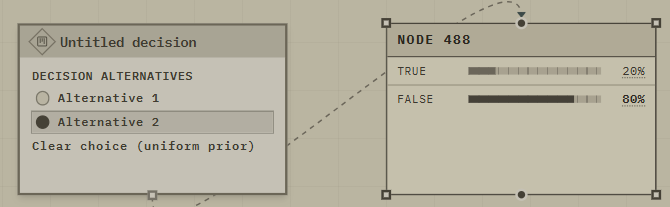
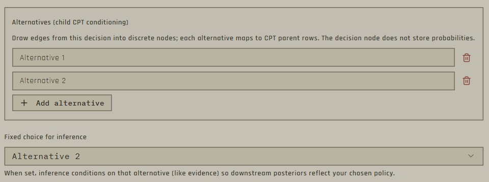
What it does: Locks which action is currently taken, or leaves the decision open. This is basically the equivalent of setting up a state for normal nodes.

Why use it: Lets you compare “if we Investigate…” versus “if we Clear…” under the same evidence.

Evidence over time (temporal)

Where to find it: Right-click a node inside a temporal plate → Observe evidence…

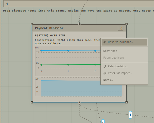
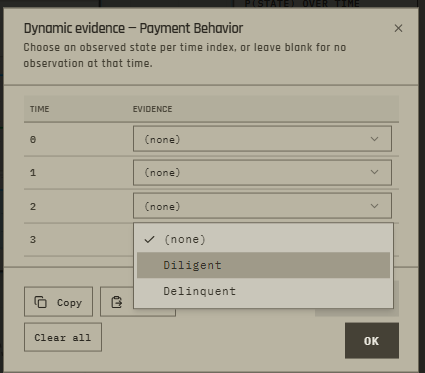
What it does: Set different observations at different time steps.

Why use it: Supports sequences: what we knew on day 1 versus day 5. You can now answer questions such as “Given a customer miss their second payment, what is the probability that they completely default on the third and fourth payment?”.

Observations on distribution nodes

Where to find it: Distribution node sidebar → Observation (backward inference).

What it does: Enter a soft constraint on a continuous quantity or on its average/spread. InferTheta updates related discrete parents accordingly.

Why use it: Lets you use numeric measurements without forcing everything into crude Low/Medium/High labels first. This is also incredibly useful for what-if simulations.

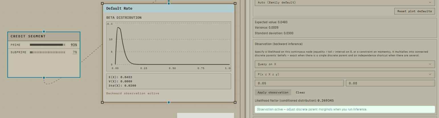
Example: The default rate below is modeled using a beta distribution, and is conditioned on the customer segment (prime or subprime). Forward inference is observing that a customer belongs to the prime segment, and thus now the expected value of the default rate drops from 7% to 4%.

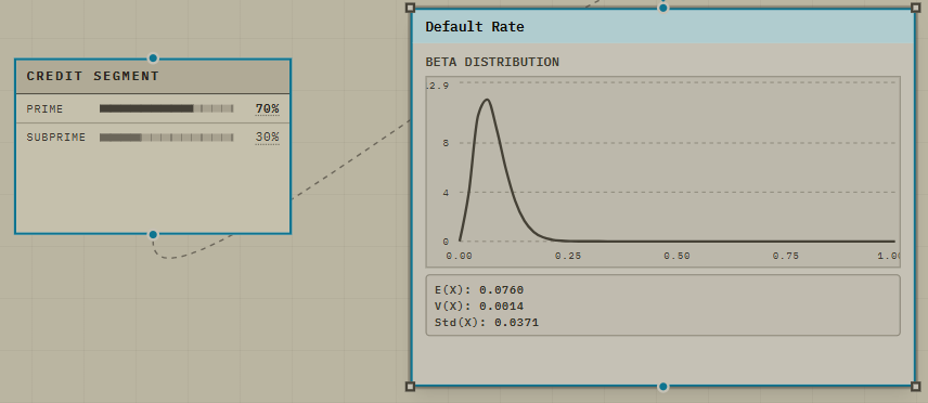
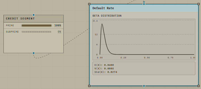
But Infertheta lets you also make backward inference on probability distributions connected to a network. You can for instance asks “If I estimate the default rate is between 5% and 8%, to what segment this customer belong to?”, which here the networks tells you there is 93% it’s a prime client.

Auto-trigger rules

Where to find it: Chance node sidebar → Auto-trigger.

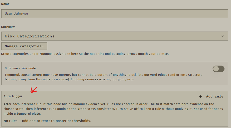
What it does: If another variable’s probability crosses a threshold, automatically set evidence on this node.

Why use it: Encodes policies like “if fraud probability exceeds 80%, treat Review as required.” This essentially forces a node to become 100% because past a certain threshold, you consider the risk too high and to make sure the model takes that into account.

Scenarios

Where to find it: Toolbar scenario dropdown, plus Create / Update / Rename / Remove.

What it does: Named snapshots of the current evidence setup. Switch between them without re-clicking every observation. Scenarios are saved with the network.

Why use it: Compare “mild case”, “severe case”, and “baseline” in one click during meetings. Again, very useful for switching between what-if simulations.

Inference schedule

Where to find it: Toolbar → Inference mode.

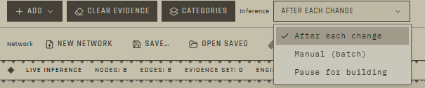
What it does: After each change: recalculate immediately. Manual: you decide when to click Run inference. Pause for building: hold updates while you draw, then run when ready.

Why use it: Keeps the interface responsive on larger models and lets you batch changes during construction. This is mainly useful when using the webapp interface. When editing very large models, if inference is not instantaneous anymore, it’s probably better to pause the inference while building, and reactivate it once done for a smoother experience.

Why the percentages on a node can differ from the CPT

Where to find it: Compare a node’s on-canvas percentages (or bar chart) with its Conditional Probability Table (CPT) in the sidebar or CPT editor.

What is going on: The CPT is local knowledge — “if the parents look exactly like this row, here is how the child is distributed.” The percentages you see on the node after inference are usually beliefs after combining the whole network with your current evidence (and any fixed decisions). Those two numbers answer different questions.

Lending example. The CPT for Default risk might say: given Employment = Unstable and Payment history = Missed payments, P(Default = High) = 70%. That 70% is only for that exact parent row. On the canvas you might see Default = High at 35% because:

• You have not fixed the parents — InferTheta averages over how likely each parent combination is right now (law of total probability).
• You set evidence elsewhere (for example a related risk flag), which changed the parents’ beliefs, which in turn changed Default.
• A decision is fixed or left open, which also reshapes downstream beliefs.

Root nodes (no parents) show their prior until something related is observed. Nodes with hard evidence show 100% on the observed state. Use Probability provenance (the control on a displayed probability) to see the mix of CPT rows that built the number on screen.

Why this matters: Stakeholders sometimes think “the table says 70%, why does the box say 35%?” The table is the recipe for one parental situation; the box is the current overall belief. Both can be correct at the same time.

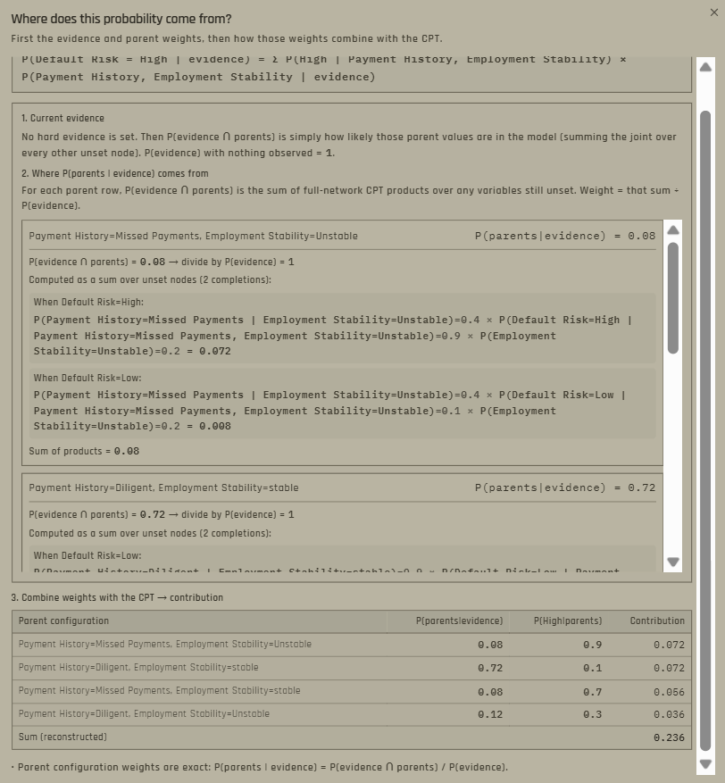
Remember, you can always click on a probability of a node (the actual %) to check a total breakdown of how the software got this number. This is why this type of approach is incredibly useful for compliance and audits. Everything can be retraced and explained mathematically.

How inference works (in one paragraph)

Inference is the process of updating every node’s beliefs so they stay consistent with the graph, the CPTs, and the evidence you entered. InferTheta propagates information along the arrows (and backwards when evidence is on a child) using the rules of probability. You do not edit those updates by hand — you change evidence, decisions, or tables, then let inference refresh the display (immediately, or when you click Run inference, depending on the Inference schedule).

Probability provenance

Where to find it: Click the provenance control on a displayed probability (the dotted % / help control on a state).

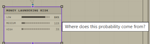
What it does: Shows a plain breakdown of how that percentage was obtained from parent situations and the probability table.

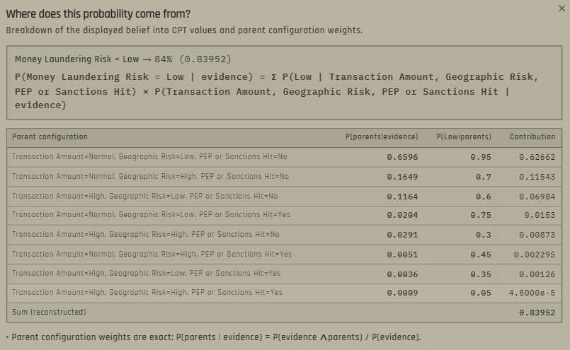
Why use it: Explains the %-bar on a child node: it is the sum of small pieces, each = (how likely this parent combo is) × (what the table says for that combo). Stakeholders see which parent situations drove the result.

6. Learn from data

You can build tables by hand, or let InferTheta estimate them from historical data. You can also ask it to propose the edges themselves. Supported file types include CSV, Excel, and Parquet. Other types of data format can be handled on demand.

For webapp users, data and relationship learning is only available for discrete nodes and Markov chains only. If you want the same thing for dynamic networks, please reach out.

Learn CPTs (fit probability tables)

Where to find it: Toolbar → Data Learning → Learn CPTs.

What it does: Upload a data file, choose which discrete nodes to update, and set how strongly to trust the data versus the tables already on the canvas (0–100%, globally or per node). 100% means you want the parameters to come only from the data you upload. Any other % means it will be a designated mix between the probabilities already input by hand and the ones from the data. It’s a way for you to insert expert knowledge / intuition in the model (very useful if the data set is still very small). If some cells are missing or unrecognized, you can use complete-case handling or EM (a method that carefully accounts for incomplete rows). Optionally open a results report afterward.

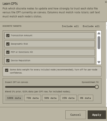
Complete-case (complete rows only)

If a spreadsheet row is missing or unrecognized for a node (or its parents), that row is skipped for learning that table. Only fully filled families count. Simple and fast; you throw away incomplete rows.

EM — Expectation–Maximization Don’t throw those rows away. Treat blanks as “unknown for now,” then guess and refine repeatedly:

• Expectation — given the current model, how likely is each possible fill-in for the blanks?
• Maximization — update the probability tables using those weighted guesses.

Repeat until it settles. Uses more of the data, but is slower and leans on your current graph/CPTs being a reasonable starting point.

Why use it: Turn spreadsheets of past cases into usable probability tables, while still blending in expert judgment when data are thin.

How probabilities are learned from data

For each discrete node, InferTheta looks at spreadsheet rows that match that node and its parents.

Count — For every parent combination (each CPT row), count how often each child state appears in the data.

Smooth (Laplace) — Add a small cushion to every count so empty cells don’t become hard 0% / 100%.

Normalize — Turn those counts into probabilities that sum to 1 for that row.

That’s the data-only table: “what the spreadsheet suggests.”

If you are learning only the CPTs (not the relationships between variables), this does mean you need to design the graph first, and make sure the name of the variables and their different states match what you have in your spreadsheet.

Format needs to be formatted this way -> First row are the names of the nodes, and the other rows their different states.

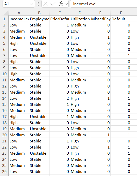
How blending with the graph works (the slider)

Before learning, the node already has a CPT on the canvas (expert / manual / previous fit). Call that the prior.

The data weight slider (0–100% data) mixes them per CPT row:

Final = (1 − w) × prior + w × data

• 100% data → use only the spreadsheet fit (prior ignored).
• 0% data → keep the canvas CPT (learning doesn’t change it).
• 50% data → halfway between expert opinion and the data, cell by cell, then renormalized.

You can use one shared weight for all nodes, or different weights per node if you’re more confident in some variables than others.

Learn Relationships (discover structure)

Where to find it: Toolbar → Data Learning → Learn Relationships.

What it does: Runs a search (CaMML / Minimum Message Length style) that proposes ranked networks — different plausible sets of edges — from your columns. You can mark outcome columns that should not point to others, tune search effort, then pick a candidate from a ranked list.

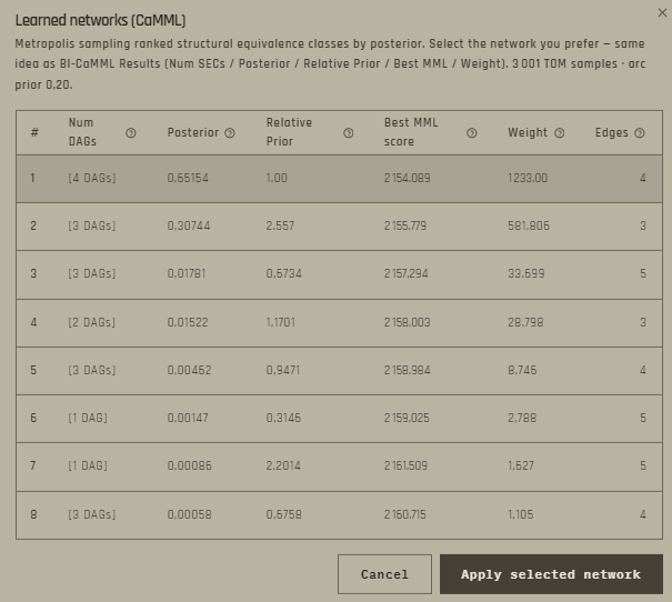
Why use it: Helpful when you know the variables but not the full dependency map, or want a data-driven starting point to review with experts.

How edges are learned

The AI does not invent probabilities first. It searches for which edges make sense between your spreadsheet columns (a set of directed edges = a network structure). You then pick one candidate; and the AI draws that graph and fits the CPT probabilities afterward. If you change the edges, always make sure to make the AI relearn the parameters!

The AI uses an algorithm called CaMML = Causal Minimum Message Length (Wallace / Bayesian Intelligence style search). Other types of causal algorithms exist and can be requested on demand for advanced users.

Minimum Message Length (MML) means: prefer a model that would let you describe the data in the fewest “bits” — short structure + good fit to the numbers. Overly tangled graphs cost more to describe; graphs that ignore the data also cost more. The sweet spot is a simple network that still explains the spreadsheet well.

• Read the columns as discrete variables (rows = cases).
• Propose many networks — try adding, removing, or flipping edges (Metropolis sampling: random walk that likes better scores and sometimes accepts worse ones so it doesn’t get stuck).
• Score each network with MML — “how expensive is this story + these tables for my data?” Lower is better.
• Group lookalikes into ranked classes (same skeleton / same essential pattern — structural equivalence).
• Show a ranked list by how much posterior weight that class got. You pick one.
• Fit CPTs on the chosen graph from the same data.

Outcome sinks (e.g. “default” / “fraud”) = columns that may have parents but must not point outward — so learning won’t treat the outcome as a cause of the inputs.

Search factor = how long the walk runs. Higher = more thorough (slower); lower = quicker, less reliable ranking.

Structure review after learning

Where to find it: Special review chrome that appears automatically after you apply a proposed network.

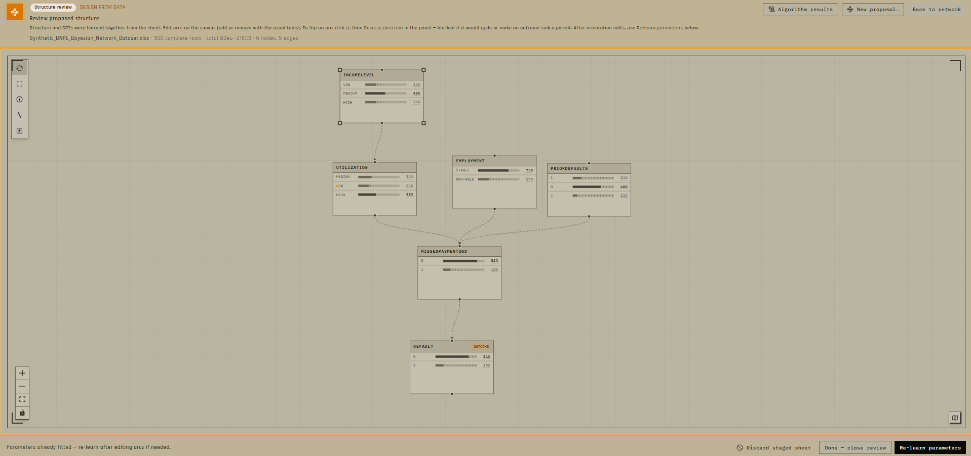
What it does: Edit arrows, re-fit tables from the staged data file, open the learning report, discard the staged sheet, or start another proposal. This is the opportunity for you to review the direction of the edges (do they make sense, or should they be reversed?) and draw new ones if necessary. Again, if you change anything regarding the edges of the network, make sure to tell the algorithm to relearn the probabilities by clicking on the “Re-learn parameters” button on the bottom right corner of the screen. If no changes are needed, you can just click on “Done - close review”.

Why use it: Keeps a human in the loop: algorithms suggest, you decide what enters production.

Learning results report

Where to find it: Dialog after learning (when review is enabled), also reachable from structure review.

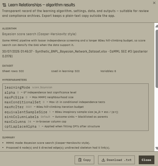
What it does: Summarizes the method, settings, data used, and per-variable outcomes. You can copy or download the text.

Why use it: Supports auditability and hand-offs (“here is exactly what we learned and how”).

Markov chains from data

Where to find it: Floating Markov chains panel (appears when Markov states exist).

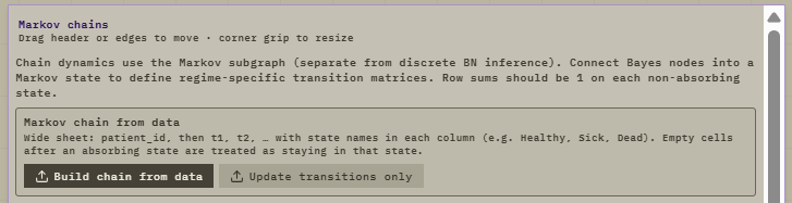
What it does: Learn or edit transition probabilities, run forecasts over steps, inspect absorption and visit statistics, and optionally use different transition tables depending on Bayesian evidence.

Why use it: Estimate how processes move over stages from historical pathways, then explore scenarios.

7. Decisions, utilities, and recommended actions

When your diagram includes at least one Decision and one Utility, you can score each possible action under the current evidence and state of probabilities.

Expected utility panel

Where to find it: Panel under the canvas when an influence-diagram setup is present. Make sure the utility nodes have a common decision node as parent for it to work correctly!

What it does: Shows a score for each decision alternative, highlights the best one, and can apply that optimal action for you.

Why use it: Turns “what might happen” into “what should we do?”, balancing likelihoods with costs and benefits you defined.

Utility configuration

Where to find it: Select a Utility node → sidebar.

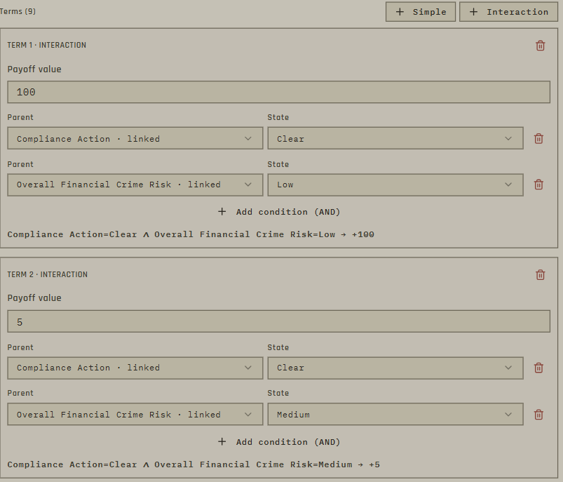
What it does: Define a baseline plus terms that add or subtract value depending on decisions and chance outcomes (including interactions).

Why use it: Encode business preferences explicitly: false alarms cost X, missed fraud costs Y, and so on.

Agent policy

Where to find it: Toolbar → Agent policy.

What it does: Write free-text context for automated assistants, plus simple threshold rules (if probability of state exceeds a level, recommend an action). These travel with JSON and Python exports.

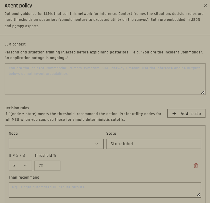
Why use it: This is very important when an external agent or workflow will call your model and needs clear operating guidance.

8. Save, share, export, and governance

Import Network JSON

Where to find it: Toolbar → Import.

What it does: Loads a full InferTheta model file onto the canvas.

Why use it: Share models across computers and teammates.

Export

Where to find it: Toolbar → Export.

What it does: Download Network JSON (full backup), or generate code for Python (pgmpy), R, C, or C++ so the model can run outside the editor.

Why use it: JSON for collaboration inside InferTheta; code exports for production systems, analysts, or embedded use.

Documents (attachments)

Where to find it: Toolbar → Documents.

What it does: Attach PDF, Word, or text files to the model (with size limits). They travel inside Save/Export JSON. You can download or remove them later.

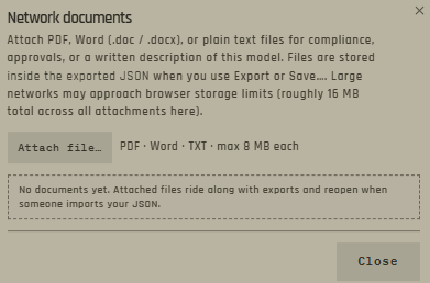
Why use it: Keep supporting material — policies, approvals, methodology notes — bundled with the model itself. Can be very important for compliance purposes.

Audit trail

Where to find it: Toolbar → Audit.

What it does: An append-only history of structural changes, table edits, learning runs, and related events. Datasets used for learning can be stored by reference. You can filter, inspect and export the trail.

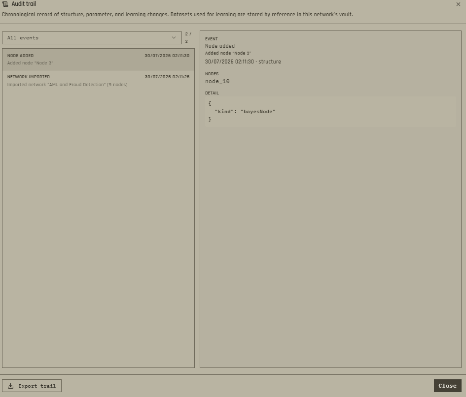
Why use it: Answers “what changed, when, and from which data?” for compliance and peer review.

9. Appearance (UI themes)

UI theme picker

Where to find it: Toolbar → UI.

What it does: Switches visual skins only. Buttons and features stay in the same places; colors and fonts change.

Why use it: Personal comfort or presentation preference without changing how the model works.

10. A simple first workflow

If you are brand new, try this path:

• Click New network and give the model a title.
• Add two or three chance nodes that matter for your question (for example Weather, Traffic, Late to work).
• Draw edges from causes to effects.
• Open each node’s sidebar and set clear state names; adjust the probability tables if you have opinions.
• Click a state to set evidence and watch other probabilities move.
• Create two scenarios (for example “Sunny” vs “Rainy”) and switch between them.
• Export Network JSON so you have a file backup.
• When ready, try Learn CPTs with a small spreadsheet whose column names match your node labels.

11. Glossary (plain language)

• Bayesian network / Probabilistic Graph (Same thing) — A diagram of uncertain variables linked by influence arrows, with rules for updating beliefs when new information arrives.
• Node / variable — A box on the canvas; something that can take different values.
• State — One possible value of a discrete variable (Yes, No, High, …).
• Edge / arrow — A directed link meaning “this helps explain that.”
• CPT (conditional probability table) — The table of “if parents look like this, how likely is each child state?”
• Evidence — Information you treat as known for now (an observed state).
• Posterior / belief — The updated probability after taking evidence into account.
• Prior — Beliefs before new evidence (often the tables as drawn or learned).
• Inference — The calculation that updates probabilities given evidence.
• Influence diagram — A network that also includes decisions and utilities (payoffs).
• Expected utility — The average score of an action under uncertainty; higher is better if you defined scores that way.
• Scenario — A saved set of observations you can reopen later.

12. Closing note

InferTheta is designed so domain experts — risk officers, credit analysts, engineers, operators — can collaborate on transparent models without needing to become statisticians first. Start simple, name things clearly, document what states mean, and only add learning or decision layers when they earn their keep.

If something on screen is unclear, use the tooltips on buttons and the Audit / Learning reports to see what the software just did. The goal is always the same: better questions, clearer assumptions, and decisions you can explain.